IITSoftware
Engineers
StanfordData
Scientists
Harvard
Data
Scientists
MITLearning
Facilitator
KPMGFinancial
Experts
E&Y Financial
Experts
DeloitteSystems
Experts
100+Customer
Engagements

Jothi Periasamy

Ramamoorthy Ramasamy

Scott Coffin

Richard Garnick

Dr. Harpreet Singh

Dr. Arivudainambi

Dr. S. Dharmaraja

Brian South

Durga Prasad

Karthikeyan Rajamanickam

Sankar Janakiraman

Bhagya Siri (IIT)

Mrithula Jothi
AI for enterprise projects have been misconceived and approached as academic concepts or scientific solutions, which has prevented businesses from realizing quick and repetitive value from AI. Many AI projects have failed to meet expectations, in great part due to lack of cross-functional skills from business process, data, AI models, Technology & Execution. Typical AI project teams comprise, at best, experts in specific areas of AI, such as AI Modelling and technology. AI projects are then executed as silo projects without any interoperability between them. In most cases, AI products and solutions are developed as use cases or as POC’s (proof of concepts) and have not been implemented as scalable enterprise solutions.
Hundreds of abstract presentations and high-level demonstrations of AI are routinely made at various venues, but we rarely see a proven AI solution for a specific enterprise.
In summary, it is a great challenge to implement enterprise-scale AI solutions for businesses. We lack scalable, repeatable and controlled AI implementation framework, processes, tools, technologies, and expertise.
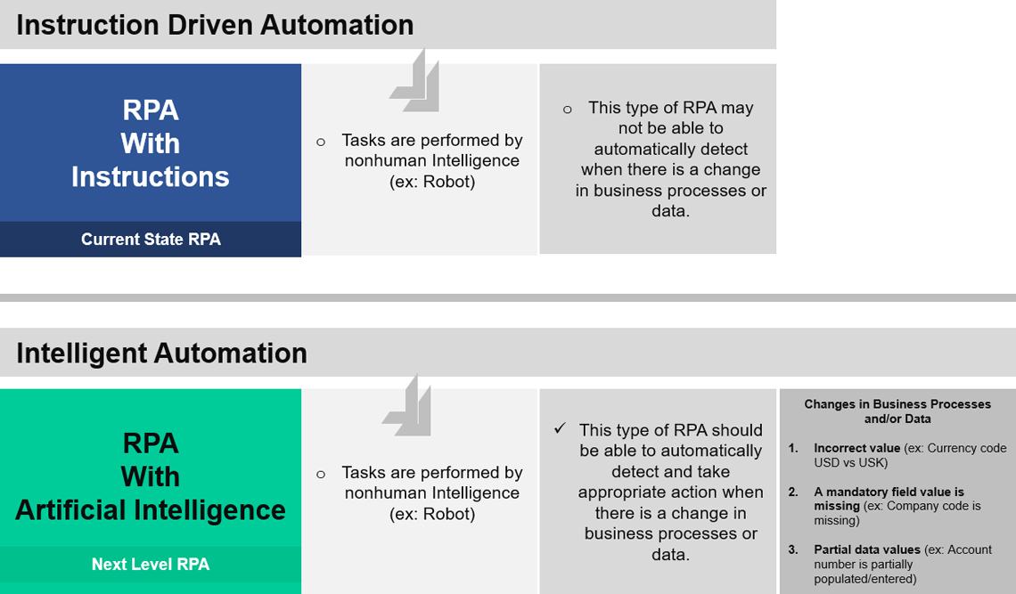
Just because a task is performed by a nonhuman intelligent process, does not mean that it is intelligent automation.
Current State - Instruction Driven Automation. If the automation of a Business Process is Instruction Driven, detection and appropriate action is to be taken when there is a change in Business Processes or Data, such an automation is called Instruction Driven Automation.
Next Level-Intelligent Automation. If the automation of a Business Process is self-driven, (without human intelligence), then detection and appropriate action is necessary when there is a change in Business Processes or Data, such an automation is called Intelligent Automation.
In this White Paper we are demonstrating AI implementation through a financial process commonly used by every business in the world - financial close. This White Paper helps the reader gain deeper knowledge on how to design, build, test and deploy AI solutions for an enterprise. Users will gain hands-on cross-functional skills, starting from the financial close process to data engineering to model building to model training & testing to model validation to model deployment.
Also, this white paper educates the users on various technologies and architectural components required to implement an enterprise AI solutions - Big Data, IIoT, AI and Cloud technologies.
Finance Transformation can defined in several different ways by industries and financial experts. From DeepSphere.AI point of view, its defined as an initiative to transform and optimize existing financial processes to meet business goals and objectives. Typically, the Finance Transformation initiatives redefine financial processes and automate them through technology.
Financial Processes:
In this White Paper, we are demonstrating the steps to reinventing financial close processes using Artificial Intelligence. We are showing the path to intelligent automation of accounting rules through machine learning and deep learning models. Our proven AI platform simplifies and digitizes financial processes.
All companies, whether small, medium or large, must declare their financial statements to their stakeholders and shareholders on time during financial period. Typically companies take two weeks to close their financial period. During financial consolidation, companies perform several key steps, including data collection from a subsidiary, intercompany matching, intercompany elimination, and financial reporting.
(ex: DeepSphere.AI, Inc. USA)
(ex: DeepSphere.AI, Inc. Germany)
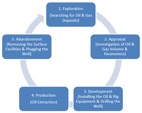
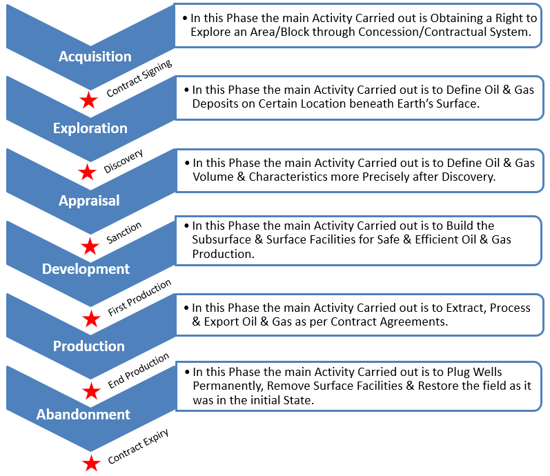
The following diagram explains the activity based life cycle of an Oil & Gas field, right from legally acquiring the block till legal abandonment (after all the economically feasible reserves are extracted) of the field.
A typical Oil & Gas E & P (Exploration and development) company incurs revenues in the production stage, rest of the stages involves CAPEX or operational expenses. Typically total Life cycle of the field is in the range of 20-50 years (Sometimes it may go more than 60 years). Out of all the stages, Highest cost is involved in the development stage. Typical development stage last for 5-10 years and the cost may go up to 10-100 Billion Dollars, if it is an offshore field.
An Activity based Life Cycle of an Oil & Gas field, right from legally acquiring the block till the legal abandonment (after all the economically feasible reserves are extracted) of the field.
Exploration: This phase consists of Identifying location for Oil & Gas deposits, using technologies like Seismic Surveys & Drilling Wells Strategically, sometimes blindly after analyzing the seismic data. In this Phase Vital Information about the Rocks, Fluid Samples etc. are Collected to Assure that Hydrocarbon is Present in the Location or not (Huge Uncertainty in the Quantity of Hydrocarbon Present still Persists in this Stage. This Stage is also Called as the Discovery Stage.
Appraisal: The main purpose of this phase is to reduce the uncertainty in the quantity of hydrocarbons present in the oil field (Reduce CAPEX Risk). In order to reduce this uncertainty, wells are drilled and more information about the field is gathered. Ex: Information about the Rocks, Fluid Ability etc. After Successful Appraisal the Company Proceeds to the Development Phase.
Development: This phase Involves designing the oil field, production facilities, export mechanisms as well as drilling optimal wells to recover the reserves. This Phase Involves Huge Cost & CAPEX and typically lasts for 5 to 10 Years.
Production: In this phase, hydrocarbons are extracted from the wells. The Life of a Typical Production Stage may Vary from 10 to 50 Years depending upon the size of the Oil & Gas Field. During this phase, revenues come in the lifecycle and expenses Incurred in this phase come under Operational Expenditure.
Abandonment: This is the phase where all the facilities are removed and the sites are restored. This is done when all the Economical Reserves are extracted from the field & when the Production Operations are no Longer Profitable.
The Following Diagram Represents a Company’s Legal Entity Structure (Company’s Operating Model). In this Model the transaction that took place between the Parent Company & the Subsidiary Company is Called Intercompany Transaction & this Transaction Should not be Included in the Company’s Consolidated Financial Reports & Should be Removed or Eliminated.
| Step One |
Step Two |
Step Three |
Step Four |
Step Five |
Step Six |
| Business Processes | Business Processes | Business Processes | Business Processes | Business Processes | Business Processes |
| Collect Subsidiaries Data: Collect Financial Data (Actuals) from Subsidiaries for the Period that you are Planning to Close. | Perform Balance Sheet Validation: For the Period that you are going to Close, Determine Whether the Balance is “In Balance or Our Balance” | Intercompany Matching: If there is any Difference in the Intercompany Booking Between the Parent Company & its Subsidiary (Ex: AP! = AR due to foreign Currency Valuation. | Intercompany Booking: If there is any Difference in the Intercompany Booking Between the Parent Company & its Subsidiary (Ex: AP! = AR due to foreign Currency Valuation. | Intercompany Elimination: Reverse the Intercompany Transactions that took Place Between the Parent Company & the Subsidiary (Ex: AR to –AR, - AP to +AP ) | Disclose the Financials: Consolidated Balance Sheet & Income Statement |
| Human Intelligence Tasks | Human Intelligence Tasks | Human Intelligence Tasks | Human Intelligence Tasks | Human Intelligence Tasks | Human Intelligence Tasks |
|
|
|
|
|
|
1 |
2 |
3 |
4 |
| Data Challenges |
Accounting Challenges |
Human Challenges |
Business Challenges |
|
|
|
|
|
|
|
|
There are Several Reasons why a Business Wants to use Artificial Intelligence in their Financial Close Processes. Here are the Key Reasons for a Business to Consider Artificial Intelligence in their Financial Close Processes:
When comparing traditional approaches with AI approach, there is a significant difference in time, cost, resource and productivity. Therefore, a business needs to use AI to achieve all of company's objectives.
| Traditional Approach | AI Approach (Sample Data) | |||||||||||||||||||||||||||||||||||||||||||||||||||||||||||||||||||||||||||||||||||||||||||
|
|
|
We have developed several Machine Learning and Deep Learning models to intelligently automate the financial close processes of a business. Here are some of the Key Financial Close Processes that we Automated through Artificial Intelligence:
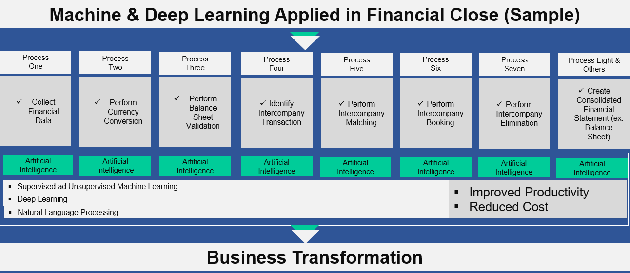
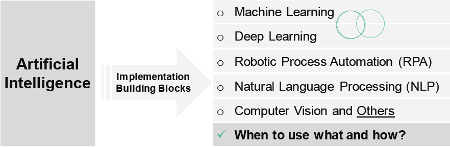
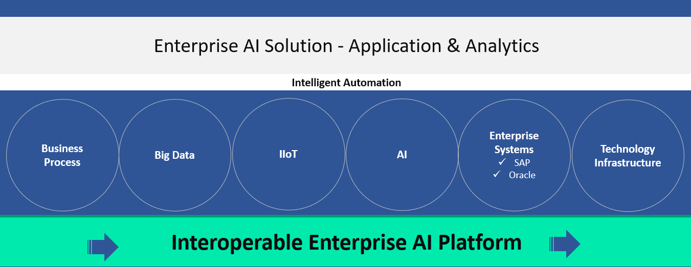
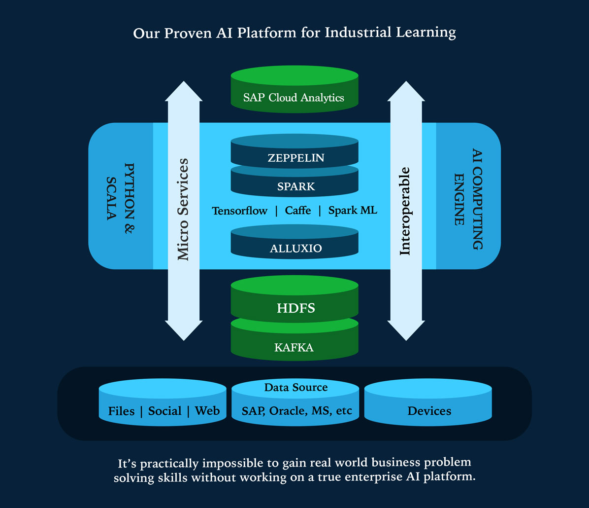
Our Enterprise AI Transformation involves implementing Machine Learning (ML), Deep Learning (DL), NLP (Natural Language Processing), RPA (Robotic Process Automation) and others. The type of automation and application we implement, entails some or all of the building blocks.
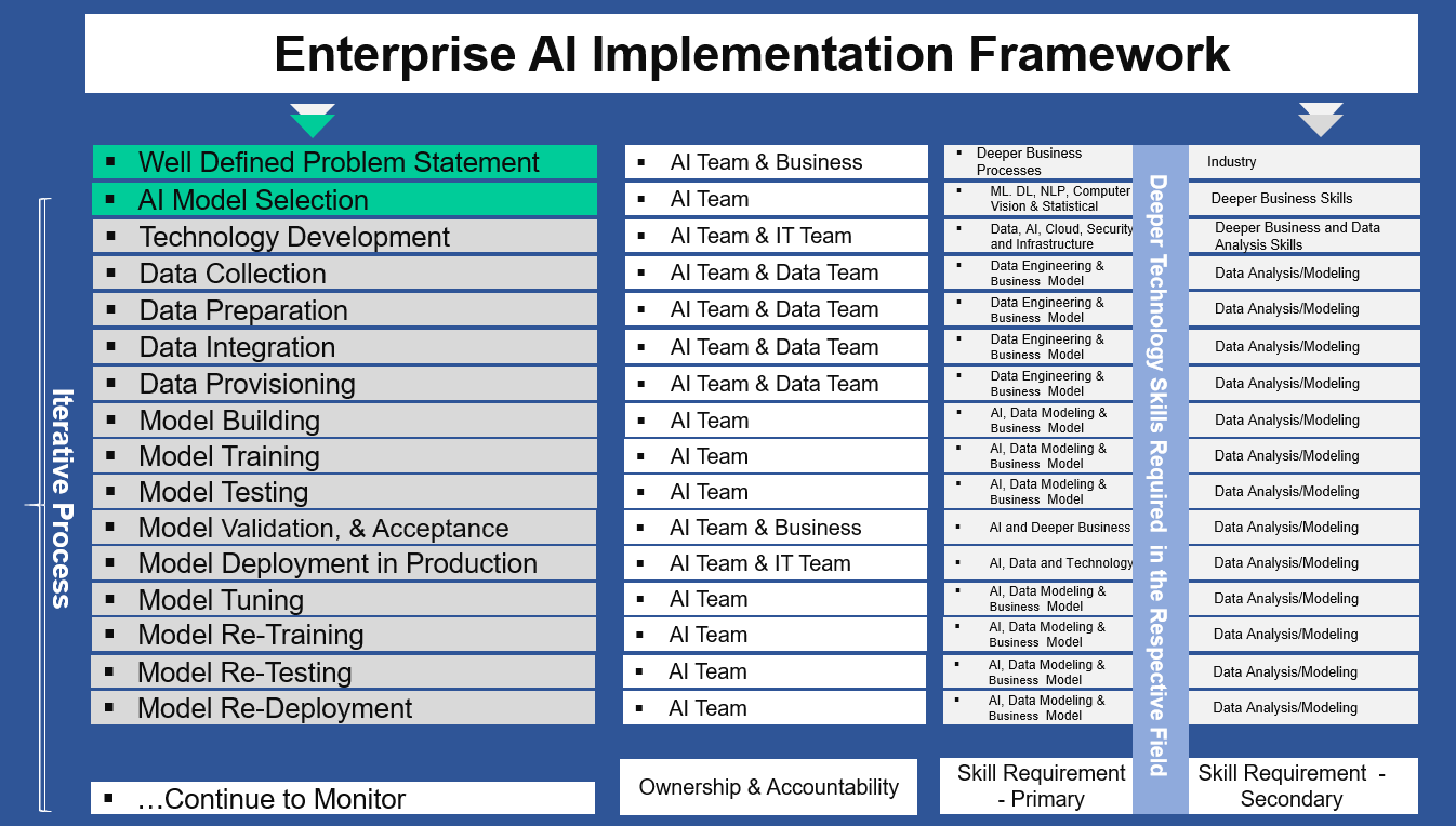
Our Proven Enterprise AI Implementation Framework enables an enterprise to automate Business Processes quickly with controllable steps by optimally managing the development efforts. Our AI Framework starts from Business Process Transformation through Data Engineering and AI Modelling. Also Our AI Framework is developed using Microservices Architecture with Interoperability to enterprise systems like SAP S/4 HANA, Oracle, Microsoft & legacy.
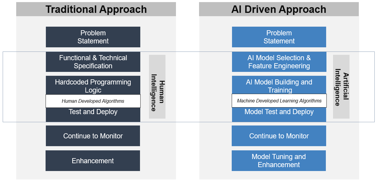
In a traditional software development approach, humans are the ones who develop the source codes based on the given functional and/or technical specifications, whereas in an AI-based approach, the machine develops the learning algorithm based on the patterns (Business Rules) that it has seen in the Dataset.
The first and the most critical step in implementing artificial intelligence for enterprise is deeply understanding the business process and translating them into a problem statement and then identifying the type of problem that we are attempting to solve using artificial intelligence.
Typically, during the design phase the AI solution, the design team takes a business process and then divides them into smaller problem statements (tasks) and expect each problem statement to produce its outcome.
Here is an example of the financial close process and how it’s divided into smaller manageable problem statements and its problem type.
# |
Business Process |
Problem Statement |
Problem Type |
1 |
Financial Close |
Identify whether the given transaction is an intercompany transaction or not |
|
2 |
Financial Close |
Determine the completeness and the accuracy of a financial transaction |
|
3 |
Financial Close |
Pair AP (accounts payable) transactions with it’s corresponding AR (accounts receivable) transactions |
K-means Clustering |
The problem type will allow us to choose the right AI model to implement and here is an example
# |
Business Process |
Problem Statement |
Problem Type |
Model Selection (Sample) |
1 |
Financial Close |
Identify whether the given transaction is intercompany transaction or not |
Classification |
Logistic Regression |
2 |
Financial Close |
Determine the completeness and accuracy of a financial transaction |
Regression |
Linear Regression |
3 |
Financial Close |
Pair AP (accounts payable) transactions with it’s corresponding AR (accounts receivable) transactions |
Clustering |
K-means Clustering |
Enterprise AI architecture is beyond building machine learning and deep learning models and it involves developing several architectural components and making them to communicate with each other. Enterprise AI architecture starts with business process architecture, then data architecture, and then AI and technology architecture.
Enterprise AI Architecture Key Components:
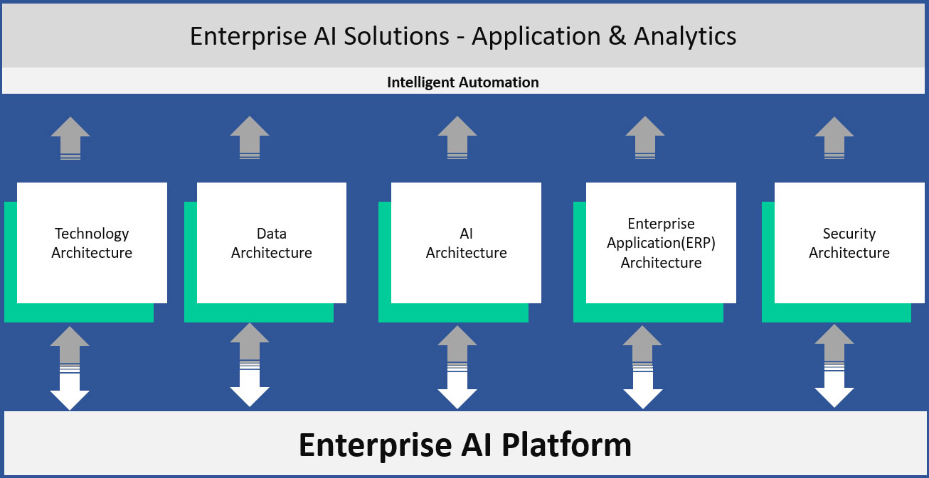
An enterprise AI solution requires a robust and a well developed enterprise architecture and an enterprise AI architecture involves business processes, big data, industrial internet of things (IIoT), machine learning/deep learning, enterprise system(ex: SAP, Oracle, etc.), technology infrastructure and security.
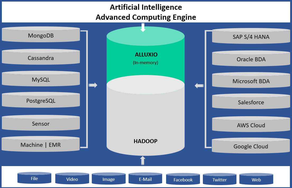
A data architecture for an enterprise AI should be able to collect, process and store data regardless of data structure, data format, and data frequency. Enterprise AI data architecture should enable ETL (extract transform and load) processes through machine learning techniques to implement instead of traditional a ETL approach with hard coded data rules.
Data Architecture Key Capabilities:
FunctionalFor our AI test drive, we have developed an advanced data platform to store and process very large data sets with a built-in connector to several data sources, including
If you are developing an enterprise AI business solution or intelligent automation, then you may consider developing a data platform through machine learning techniques instead of traditional hardcoded data rules.
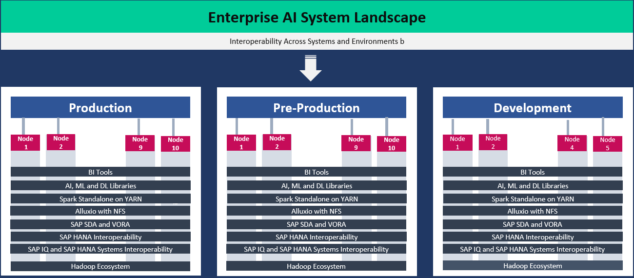
An enterprise AI technology infrastructure should be built on modern architectural components such as CPU, ManyCore processors, GPUs, FPGAs, and ASICs with interoperability to existing legacy systems.
An enterprise AI technology architecture should be flexible and open to support various business solutions and should not be developed for a particular use case or a specific solution.
For our AI test drive, we have developed an architectural framework to support current (ex: financial close) and future (ex: planning, forecasting, analytics, and etc.) business needs.
Adopting microservices for data engineering and model engineering is an important architectural decision. Microservice increases the reusability of code block and also it enables loosely coupled services to be called across AI models and across AI solutions.
Key Microservices
Loosely coupled services to quickly deploy Artificial Intelligence at an enterprise scale

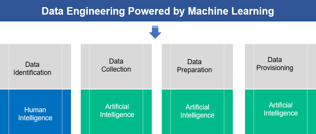
From AI perspective: Data identification is an effort to identify relevant and required data for business process automation, business reporting, business analytics, and/or business data analysis. This effort includes the following key tasks
From Financial close perspective: Identification of relevant data that’s required to close the book and disclose the financial statements.
Example:
From AI Perspective: Data collection is collecting training and test data from various sources to perform key tasks such as AI model building, training and testing activities. Typically, data collection is part of data engineering and the key task that’s involved are
From Financial Close Perspective: Data collection is collecting the subsidiaries financial data from different sources to a centralized data storage to initiate the financial close processes.
From AI Perspective: Data comes in different formats from various sources, data preparation integrates the data for AI model training and testing. Instead of traditional ETL process, we use machine learning techniques to prepare the training data sets and test data sets. To prepare training and test data for the model, traditional ETL process may not be an option as data changes when there is a change in the business process that’s why we use machine learning technique for data preparation so that the machine learns and understand the changes in the data and its pattern. Below are the tasks without any hardcoded data mapping rules for data engineering function
From Financial Close Perspective: Data collection is the final step to make the data available to the financial close process to start. During this process typically several data mapping activities take place and typically these tasks are performed through hardcoded instructions/rules.
Example:
From AI Perspective: During the development phase, data provisioning process supplies train and test data on a timely manner for model training and testing. During Production, data could be made available to the model based on business transaction occurrences, business event occurrences, and/or during initiation of a business processes.
Example:
From Financial Close Perspective: For the close process to run financial data is made available on Real-time or defined frequency basis (ex: daily, weekly, monthly, etc.). These types of tasks are performed traditionally through standard ETL process and we in this white paper are demonstrating how these are performed using machine learning techniques.
In this section, we are providing steps, processes, tools and technologies to implement AI models - Machine Learning and Deep Learning.
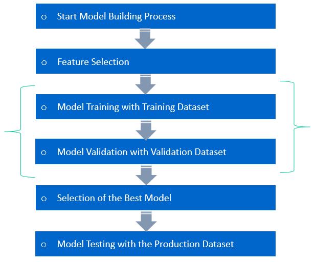
Model Selection is a task of selecting between various machine learning algorithms. The selection of a model could be seen as a low priority option, but there lies a Best Model/algorithm for a particular problem.
Example: When performing Intercompany Transaction Identification (Transaction is intercompany or external), there are a number of model/algorithms that would help us achieve the desired result. We can either use Logistic Regression algorithm, Support Vector Machines algorithm, K-Nearest Neighbor algorithm, Decision Tree algorithm, and Random Forest algorithm. The complexity lies in choosing the best model for the prediction. Each of the models must be tested individually or placed together in a Machine Learning Pipeline and verified for accuracies. This whole task is termed as a Model Selection Process.
The Best Model Selected meets the following Objectives:
Feature Engineering is converting a raw dataset into more appropriate feature set that better Represents the underlying problem to the predictive models. Feature Engineering, a painstaking task, becomes difficult with large dataset and requires domain specific knowledge to identify the best features for the model. Good features enhance the performance and efficiency of the predictive models. Thus, even when the machine learning task is similar in different scenarios, the selection of features in each scenario is specific to a specific scenario.
Feature Engineering is an important part of Building an Effective & Result Oriented Solution. Even when there are lot of Other Methodologies like Deep Learning which Facilitate Automated Feature Selection task, better feature selection acts as one of the main core task that decides the performance of the underlying Model. It is Regarded as a Phenomenon where a Resource Spends most of time in Data Preparation before modelling. Feature Engineering acts as a task that decide between Success & Failure of a Project.
Example: During Intercompany Validation, the Raw Dataset for Model Building needs to contain only the Required Feature Set. Of these feature set, only the features that serves our purpose are taken into account. This is a Process of Feature Engineering & Feature Selection.
Feature Engineering enables the following:
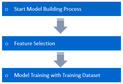
Model Development is nothing less than building of a product itself. It Involves Process of Training, Validation & Testing. The Model is just an empty brain with inbuilt logic for prediction. Training Data is to be fed to the Model so that the model learns the Patterns in the dataset.
Machine Learning operates on a principle of finding relationships between a label its features. We Show the Model with many examples from our Dataset to understand the relationship between the Label and its features thoroughly. In other words, it memorizes the entire input dataset perfectly. This Process is called Model Training.
Let’s take an example of the Intercompany Transaction Identification, create a model from a logistic regression estimator. The model gets the Logistic regression Data through the fit function. Then we pass in a test set of features through the predict function. The model outputs an answer based on its training.
Model Testing refers to testing the model with the Test Dataset. The Model is trained with Training Data for Learning the Patterns in the Dataset and validated against the Validation Dataset, then tested with the data never seen. This process is referred to as Model Testing.
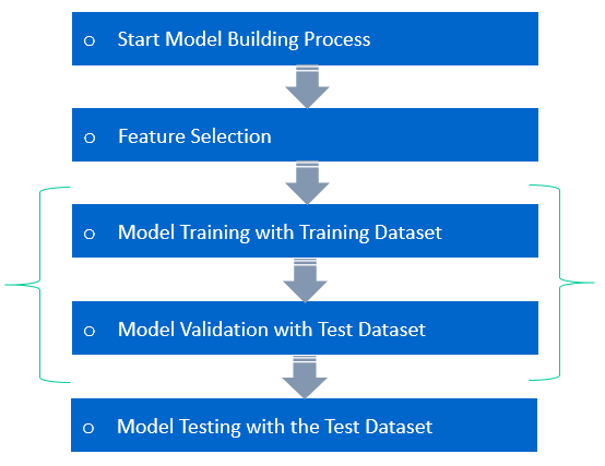
In Machine Learning Model Validation refers to a process in which a trained model is validated against a Validation Dataset. The Validation Dataset is a separate section of the same data set from which the training set is derived. The main advantage of using the Validation Dataset is to test the generalization ability of a trained model. Model validation is performed after model training. Along with model training, model validation aims to find an optimal model with the best performance.
Fitting is a measure which tells us how the model generalizes on the unseen data, based on the learning it underwent during the training process. A Model that is Regular Fit produces an accurate outcome. A model that is underfit underperforms as it has learned the patterns in the data poorly. A model that is Overfit over performs, or it has modeled that too closely.
Fitting is the root of machine learning. If our model does not fit well, the produced outcomes are inaccurate to be useful for a practical decision making process.
Regular/Best fit is a case when the model performs well on unseen data & generalizes very well. Ideally it makes Zero Prediction errors. This Sweet spot of Generalization Occurs between spot of underfitting & Overfitting. In order to understand it we will have to look at the performance of our model with the passage of time, while it is learning from training dataset.
Fitting is a measure which tells us how the model generalizes on the unseen data, based on the learning it underwent during the training process. A Model that is Regular Fit produces an accurate outcome. A model that is underfit underperforms as it has learned the patterns in the data poorly. A model that is Overfit over performs, or it has modeled that too closely.
Fitting is the root of machine learning. If our model does not fit well, the produced outcomes are inaccurate to be useful for a practical decision making process.
Under Fit is a case in which the model performs poorly on the unseen data and does not generalize. This happens because the model does not capture the relationship between the Label & the Features properly. Also the Training Dataset could be small.
Fitting is a measure which tells us how the model generalizes on the unseen data, based on the learning it underwent during the training process. A Model that is Regular Fit produces an accurate outcome. A model that is underfit underperforms as it has learned the patterns in the data poorly. A model that is Overfit over performs, or it has modeled that too closely.
Fitting is the root of machine learning. If our model does not fit well, the produced outcomes are inaccurate to be useful for practical Decision Making Process.
Over fit is a case when the model performs well on the seen data and poorly on the unseen data. The model does not generalize well. This happens because the model memorizes the dataset it has seen & unable to generalize on the unseen samples.
When developing a Machine Learning model, we have choices to define model parameters. Often some of the undefined parameters may not produce the expected outcome. Parameters which define the model architecture are referred to as hyperparameters and tuning these Parameters is called Hyperparameter Tuning.
These hyperparameters might address the following queries:
Machine Learning models deals with Streams of Data. The Dataset it got trained for may be appended by a New Dataset that significantly differs from the one that it trained on. Then the Machine Learning Models needs to be accurate, scalable, repeatable and ready to go Kind so that it can efficiently integrate with the Information Systems.
For accurate model prediction, the data that it predicates must have a similar distribution as the data on which the model was trained. As data distributions are expected to change over time, deploying a model is a continuous process. It is a great exercise to monitor the incoming data continuously and retrain the model on newer data if you find that the data distribution has deviated significantly from the original training data distribution. If monitoring data to detect a change in the data distribution has a high overhead, then a simpler strategy is to train the model periodically, for example, daily, weekly, or monthly. This way, our predictions tend to upgrade based on the dataset you are using.
As the Model undergoes retraining, it would have learnt the patterns from the new dataset, appended on it. Hence the test dataset needs to be appended as well. The Retested Model predicts the results accurately now, as it was Re-Trained on the New Dataset. Hence, the performance of the model is upgraded.
Deploying a standalone AI use case is not a time-consuming & complex task as it involves fewer technologies and simple business processes. But, deploying an Enterprise AI Solution or an AI Application is cumbersome because Deployment involves arranging several technology components together from the Data to Enterprise Systems.
Key Challenges in Enterprise AI Deployment:
In our AI test drive, we are using several systems, libraries and interfaces and setting up these systems to intelligently automate a business process that takes more time, cost and resources. Using Docker, we can simplify some of these challenges.
Key Technologies Used in Our AI Test Drive:
Why Docker Based Deployment?
Docker is a containerization platform that packages your application and all its dependencies together in the form of a docker container to ensure that your application works seamlessly in any environment. Simply, Docker is a tool designed to make it easier to create, deploy and run applications by using containers. Containers allow a developer to package up an application with all of the parts it needs, such as libraries and other dependencies, and then ship it all out as one package. In so doing, thanks to the container, the developer can be rest assured that the application will run on any other Linux machine regardless of any customized settings that the machine might have used that could differ from the machine for writing and testing the code.
Docker is like a virtual machine. But unlike a virtual machine, creating a whole virtual operating system, Docker allows applications to use the same Linux Kernel as the system that they are running on and only requires applications to be shipped with things not already running on the host computer. This significantly boosts performance and reduces the size of the application.
These containers use Containerization, considered to be an evolved version of Virtualization. The same task can also be achieved using Virtual Machines, however it is not very efficient. There are two key parts to Docker: Docker Engine, and Docker Hub. It is equally important to secure both parts of the system. To do that, it takes an understanding of how they are comprised, which components need to be secured, and how to secure them. Let’s start with Docker Engine.
Docker Engine hosts and runs containers from the container image file. It also manages networks, and storage volumes. There are two key aspects to securing Docker Engine: namespaces, and cgroups
While Docker Engine manages containers, it needs the other half of the Docker stack to pull container images from. That part is Docker Hub—the container registry where container images are stored, and shared.
| Oil & Gas Upstream Accounting Structure | |||
| Financial Accounting Category | Financial Account | Business Context for Account Usage | Account Type |
| Explorations & Appraisal Activities | Pre-licensed Exploration activities | The organiation may choose to make the data freely available to potential investors, sell it to interested parties, or require its purchase as a condition for participation in the licensing round. | Expense |
| Post-licensed Exploration activities | After winning a bid, the company sometimes argues that circumstances have changed and the project is no longer viable under the existing terms of the license. | Expense | |
| Farm-out expense | Farmout is the assignment of part or all of an Oil & Natural Gas or mineral interest to a third party for development. The interest may be in any agreed upon form, such as exploration blocks or drilling acreage. The third party, called the “farmee”, pays the “farmor” a sum of money upfront for the interest and also commits to spending money to perform a specific activity related to the interest. | For the farmor, the reasons for entering into a farmout agreement include obtaining production, sharing risk, and obtaining geological information. | |
| Exploration & development, acquisition costs | Cost incurred in getting the details of the field. | Expense | |
| Exploration survey costs (Seismic data acquisition costs) | Oil & Gas explorers use seismic surveys to produce detailed images of the various rock types and their location beneath the earth's surface and they use this information to determine the location and size of Oil & Gas reservoirs. The cost for further improving the data has been acquired by the organization. |
Expense | |
| Seismic data process infrastructure and costs related to it | The computational analysis of recorded data to create a subsurface image and estimate the distribution of properties is called data processing. | Expense | |
| Appraisal Drilling costs | The cost for drilling the appraisal wells for exploring the block. It also includes reservoir data. | Expense Developing a field |
|
| Costs incurred for unproven properties | If you buy a block of land and later find that it is an unproven reserve with no hydrocarbons, then the money spent in buying the land becomes the cost incurred due to no findings. | Expense Total Loss |
|
| Well costs | The cost that is incurred in drilling and completing the Oil & Gas well. | Expense, It will be an asset. | |
| Mineral interests/transfer of mineral interests | Ownership of the right to exploit, mine or produce all minerals lying beneath the surface of a property. In this case, minerals include all hydrocarbons. 1. If you want to sell the mineral rights to another person, you can transfer them by deed. You will need to create a mineral deed and have it recorded. 2. You can put mineral rights in your will. After your death, the rights will pass to the beneficiaries listed in the will. 3. If you want to lease mineral rights to a third party, then you will need to create a contract. |
Expense It will be an asset./ Transfering mineral interest might be profit or loss. |
|
| Interest In Joint Venture | A Joint Venture (JV) is a business arrangement in which two or more parties agree to pool in their resources for accomplishing a specific task. | Reason for JV: 1. Capital Intensity 2. Risk Mitigation 3. Access to Technologies 4. Access to Resources 5. Supply Chain Optimization |
|
| Land Lease expenses | It also includes land for surface facilities like Group Gathering Station (GGS), where the hydrocarbon is processed, stored, or supplied after production. | Expense | |
| Bidding costs for the blocks | Bidding cost of the block is decided by the organization and then put on auction. | ||
| Development Costs | Well costs | The cost that is incurred in drilling and completing the Oil & Gas well. Well costs depend on the well design of each well. Well cost may differ for appraisal, exploratory and development wells, because of some design change that was experienced because of the appraisal or exploratory wells. | Expense, It will be an asset. |
| Development expenditures | Development expenditures include the cost of the wells and the surface facilities required for the treatment and supply of the hydrocarbon. | Expense, It will be an asset. | |
| Asset selling or sublease | Revenue generated from selling the proven assets or leasing them. | Revenue. | |
| Intangible drilling costs | Intangible drilling costs are costs of elements required to develop the final well, such as survey work, ground clearing, drainage, wages, fuel, repairs, supplies and labor. | Expense | |
| Tangible drilling costs | The costs of Oil & Gas equipment, or tangible items, such as casing, pumpjacks, tubulars, blow out preventer, cement, etc. are deemed to be tangible drilling costs. | Expense | |
| Tangible completion costs | The costs of Oil & Gas equipment, or tangible items, such as tubing, packers, subsurface valves, perforation, wellhead, permanent downhole gauges etc. are deemed to be tangible completion costs. | Expense | |
| Intangible completion costs | Intangible completion costs are costs of elements required to develop the final well, such as or the elements that are not a part of the final operating well. | Expense | |
| Dry hole costs | All costs up to and including drilling the well and testing the presence of hydrocarbons. In addition to drilling expenditures, these include the costs for leasing land, seismic purchase and reprocessing. The primary risk to an investor's capital is drilling a well and not finding oil or gas. Dry hole costs are usually 2/3 or more of the total capital at risk in drilling a well. Once a well tests positive for hydrocarbons, the operational risk level is usually reduced. |
Expense Total Loss |
|
| Third party assurance studies (FOR DGH) | If you buy a block but you don’t have the domain expert for the field development planning, then you hire the third party for doing the required studies | Expense | |
| Production & Abandonment Operational Expenses | Coring and consequent lab studies on rocks and fluids | These studies are done to increase your knowledge of the reservoir. Coring means you take out a small portion of the reservoir rock while drlling and then test its properties. |
Expense |
| Hedging transactions | Hedging commodities allows investors to ensure predictable financial results by protecting themselves against future price movements. By purchasing futures contracts, investors can lock in prices that are favorable to an organization to continue realizing profits over time. | Protecting the company | |
| Domestic market obligation | It varies from country to country. | ||
| Cost recovery | CR is the term used to recapture a contractor’s capital expenditures and operating expenses out of gross revenues after first production under the production sharing contract. | Revenue. | |
| Production bonus | Payment by a well operator to a host country upon achievement of certain levels of production. | Expense | |
| Impairment expenses | Impairment is specifically used to describe a reduction in the recoverable amount of a fixed asset below its book value. Impairment normally occurs when there is a sudden and large decline in the fair value of an asset below its carrying amount, or the amount recorded on a company's balance sheet. | ||
| Underlift/over lift | An underlift position arises when an organization owns a partial interest in a producing property and does not take its entire share of the Oil & Gas that is produced in a period. | Revenue/ Expense | |
| Crude selling | Revenue. | ||
| Decommissioning obligation | Decommissioning of the onshore plant or the offshore platform after the life of the field. The cost varies from country to country. | Expense | |
| Production costs | The cost incurred during the production of the field. | Expense | |
| Penalties to govt & ocean cleaning charges(if blow out etc happens ) | There are charges and penalties for these depending upon the country policies. | Expense | |
| Obsolete inventory or assets | Excess inventories that can be used for future projects or sold as scraps. | Expense / Liability | |
| Field abandonment charges | Costs spent on closing and abandoning wells and making the pipelines hydrocarbon free. | Expense | |
| Cost oil | A portion of produced oil that the operator uses on an annual basis to recover defined costs specified by a production sharing contract. | ||
| Profit oil | The amount of production, after deducting cost oil production allocated to costs and expenses, that will be divided between the participating parties and the host organiation under the production sharing contract. | Revenue | |
| General Expenses | Legal expenses (in case of arbitration ) | ||
| Services offered by/ to other companies | If you buy a block but you don’t have the domain expert for ex field development planning, then you hire a third party for doing the required studies. | Revenue/ Expense |
# |
AI Terminology |
Key Points |
Business Context |
1 |
Feature engineering |
Features are properties of all/shared by all the independent variables in the analysis, which help in identifying, measuring, and understanding the occurring event. Feature engineering is about identifying all such features, using domain knowledge, which helps machine learning algorithms to predict and improve their performance. |
Many conventional analysis used for predictions like Decline Curve, IPR, P/Z analysis are all features. Using the machine learning algorithms, many processes, like these can be performed seamlessly by the machines. |
2 |
Model Validation |
The process of Validating the performance of the machine learning algorithm model against what was envisaged is called model validation. |
It has significant impact on the decision making process because better the models are better our predictions will be and hence the decisions. Useful in various Models like prosper, Decline curves,EOS models, Assisted history matching, validation of properties population in Static models with well logs etc |
3 |
Underfitting |
If the prediction model performs poorly on the training data-set (input data), then the model is called underfitted model. Assessing the model fitting gives a better idea on the usefulness of the model for the predictions. |
Assessing the model-fitting regularly will improvise the prediction process. Important phenomenon like instrumentation error (or inaccuracy ), scientifical dependency of the analysed parameters etc.., actually suggests how a model to be fitted and determines whether a model is under, regular or over fitted. Assessing the model-fitting regularly will improvise the prediction process. Eg: for analysing the decline in gas rate with time, usually gas rate vs time plot will help in giving a reasonable estimation of future gas rates, but in the wells where water breakthrough happens, the decline in gas rate also depends on the amount of water produces. So in these type of wells features dictate whether a model is under-fitted or over fitted. |
4 |
Overfitting |
If the prediction model performs well on the training data-set (input data) and doesn’t perform as envisaged during the predictions, then the model is called overfitted model. Assessing the model fitting gives a better idea on the usefulness of the model for the predictions |
|
5 |
Regular Fit |
If the prediction model performs reasonably good on both training data set and suring predictions, it is called regulat fitted model |
|
6 |
Classification problem |
If the problem involves categorization of the observation on qualitative or numerical basis, then it is called classification problem. |
|
7 |
Regression problem |
Estimating the relationship between two variables is called regression. The problem involving prediction of quantity is called regression problem. |
Useful in production forecasting, Identifying the IPR cuvre and reservoir pressure estimations using the well test data |
8 |
Univariate analysis |
If there is only one variable in the analysis, it is called univariate analysis. Central tendencies of the data, frequency, patterns in the data etc. are analyzed. It takes the data and summarizes pattern in it. Dealing with causal relationships with other variables are not considered. |
Very useful in assessing the static model properties and their population in the model. It will be used to assess the effectiveness of various operations. Once the patterns in the operations data are found, further analysis for the root causes can be completed. |
9 |
Bi-variate analysis |
As the name suggests, it analyses data with two variables. This mainly focuses on the causal relationships and dependency of the two variables on each other. |
Most used analysis (Because of the ease with which it can be done in excel, over multi variate analysis). Used to assess the effect of various wells parameters (like Pressure, temperature, pressure loss across the choke, separator pressure etc) on production rates. Used to plot Log measurements Vs Depths, Used in conventional reservoir techniques to assess the reservoir. |
10 |
Multi-variate analysis |
As name suggests, it analyzes data with two variables. This mainly focuses on the causal relationships and dependency of the two variables on each other. |
Very useful and less used in Oil & Gas Industries. Usually predicted properties like future production rates, wells deliverability, pump failures, reservoir behaviors depends upon many variables. Constraining the problem to Bi-variate analysis over simplifies the problem most of the times. So, using Multi-variate analysis combined with principal component analysis increases the effectiveness of the predictions. |
11 |
Machine Learning |
The ability of the machine to learn from the past data (By identifying the features and building algorithms), without being programmed extensively is called machine learning. |
Can be extensively used in History matching analysis, well tests to assess the reservoir performance and condition |
12 |
Types of machine learning |
supervised machine learning (need a data analyst to identify the inputs and the output to be predicted) and unsupervised machine learning (Doesn’t need analyst, need extensive data (big data) for the machine to learn from it, it uses techniques like deep learning to review data and to come to conlcusions and hence actions based on them. |
|
13 |
Cross Validation |
Machine learning models are trained with subset of actual data (called training data) and then evaluated with complimentary data sets to assess the predictability of the ML models. Very useful to assess whether the model is over-fitted or not. |
|
14 |
Deep Learning |
Deep Learning is an unsupervised machine learning technique. It is the set of learning mechanisms, machine follows to process and understand hugely available datasets. |
Sand production has always been a concern in Oil & Gas wells. Existing sand detecting equipments use acoustic and conductivity measurements to assess the sanding phenomenon, but there are many limitations to these methods. Computer vision which uses deep learning techniques can be of great value addition in this field. Main applications are sand detection during the flow, Identifying sand accumulation in field equipments like (separators, bend pipelines, tank bottoms etc) which will save time & money and great value addition for incident prevention, Screen plugging detection (to identify the formation damage or PI reduction). |
15 |
Artificial Neural Networks |
It’s a computational framework (Consisting of several nodes (called as neurons)) on which multiple machine learning algorithms work together to learn from the experience (past data). It attempts to simulate the process human brain neurons follow in aquiring the knowledge from the experiences and using it when required. ANN is a part of Deep Learning |
|
16 |
Computer Vision |
It is the ability of the machine to see and detect the objects. Using the deep neural networks and with huge image datasets makes this possible. In this technique, a computer divides the images into raster and vector images and recognizes the patterns in the image. |
Applications can be in equipment damage inspection,(drill pipes etc), Identifying the different equipments in the dockyard (Dockyard is a place where all the equipment is stored) So that even a new employee doesnt face difficulty in identifying which is what. Sand detection, Object detection systems for ROV (Remote operated vehicles). Digitising the old datas of the E & P companies. Surveillance for oil field tankers and On-shore pipeline valves from which oil can be stolen. |
17 |
Raster Image |
Pixels are the building units for this type of image. If we zoom the image clarity will be lost. |
|
18 |
Vector Image |
Polygons/pathways are building units for this image. Even if we zoom the image clarity of the image wont be lost. |
|
19 |
Outliers |
In the dataset the individual points which are distant from the other points are called outliers. Outliers may occur due to measurement error or high skewness of the data or may happen due to specific incidents. Understanding the outliers will help very much in doing statistical analysis. Should be cautious in using normal distribution when outliers are present. |
Helpful in performing every forecast and analysisng the reservoir surveillance trends, Regularly used in decline curve analysis to remove the points where measurement/allocation errors happen. |
20 |
Probability distribution |
A function describing the probability of each individual outcome of a particular event. This includes discrete probability function, continuous probability distributions (probability is a continuous number like temperature of a day). |
Useful in uncertainty analysis for inplace estimations, probabilistic estimations of different properties like porosity etc. |
21 |
Probability Density Function |
Probability distribution function of continuous variables. Instead of telling the absolute probability of a random variable directly, it describes the probability of the random variable to fall in a particular range of values. |
Very helpful in estimating in place, recovery estimations, NPT estimations, etc. Very useful for the finance department to assess the investments, ROI etc. |
22 |
Linear Model |
|
|
23 |
Time series |
A set of data points where points are indexed according to time. |
|
24 |
Normalising data |
The process of eliminating the amplitude variation in the datasets by preserving the distribution shape is called Normalizing data. Mainly useful to compare different datasets. It is better to perform normalization in order to speed up the convergence. |
Useful for normalizing the Relative permeability curves to prepare the input data for the models. Very helpful in iteration calculations, which will be used in every simulation model in the market. Useful in multivariate analysis where one independent values magnitude is high compared to the others (In this case one variable will outweigh the other due to the magnitude difference, which should not be the case always). Provides immunity to the outliers. |
25 |
Standardisation |
The process of converting any distribution to a normal distribution having a mean of "zero" and a standard deviation of "one" is called standardizing. |
|
26 |
Stationary time series |
Time series, in which data points probability distribution doesnt change when shifted over time i.e, series in which, mean,variance, coefficients and auto-correlations are constant over time is called stationary time series. Most statistical forecasting methods work on the assumption that the time series on which prediction is being done is approximately stationary. |
Most forecasts done now-a-days in the industry are done using simple regression techniques. In most of these cases the process of making the time series "stationary" is usually not followed. If used properly, this could improve the forecasts reliability. (Can be clubbed with our sick-well analysis to add other features in it like well's IPR change with time or decline estimations etc.). Currently Decline Curve analysis (gas rate time series) is being done in MBAL software, which doesn’t have robust tool-set to make the "time series. |
27 |
Non-stationary Time series |
The time series in which mean and variance changes with time, stochastically, is called as non-stationary time series. |
|
28 |
White Noise |
A discrete signal whose data points are uncorrelated random variables having a mean of zero and finite variance. It is a simple example of stationary time series. |
Useful in signal processing. Acoustic data of clampon sand detector have base line data plus background noise (noise due to subtle flow fluctuations). White noise elimination techniques are used to calculate the actual sand base line. |
29 |
Confusion Matrix |
It is matrix representation of the performance of machine learning algorithm. It basically shows the tabular representation of actual outcomes Vs predicted outcomes it shows the event-specific (or outcome) tabular report of performance, where Actual positives and negatives are plotted against the predicted positives and negatives. |
In the decline curve analysis only the data points, where operational changes (choke changes, separator pressure changes) are absent, to be considered. The identification of the points where external operations are done can be identified by Machine learning algorithms. Confusion matrix (or table of confusions) can be used to compare the algorithms performance against the actual incidents. |
30 |
Table of confusion |
While confusion matrix shows the tabular representation of all the outcomes at once, the table of confusion show the event-specific (or outcome) tabular report of performance, where Actual positives and negatives are plotted against the predicted positives and negatives. |
|
31 |
Accuracy |
A description of both random and systematic errors, i.e., It describes both precision and trueness. |
|
32 |
Collaborative filtering |
A technique to identify the patterns to draw some conclusions using multiple datasets, viewpoints. |
Usually collaborative filtering is used in huge datasets. Oil & Gas companies have huge seismic data. Collaborative technique can be used to find the prospect zones, or to estimate the attributes in a well using other wells data. |
33 |
Imbalanaced datasets |
The training dataset where one class of data is more occuring compared to the other class is called imbalanced dataset. Even though the machine couldnt predict the less occuring data, the accuracy of the prediction will be high, which leads to building a less effective model. |
Identification of rate changes and causes of it is very important for the decline curve analysis.rate changes in the wells are more frequent due to allocation and less frequently will be due to operational reasons. Having an idea on imbalanced datasets will give a better effectiveness in building machine learning models |
34 |
Categorical Variables |
Variables where each individual observation belong to limited values based on its characteristic either nominally or qualitatively. |
|
35 |
Continuous variables |
Variables having numerical values as the observations and which have infinite values between any two observations. |
|
36 |
Discrete Variables |
Variables having numercial values as the observations, and there are finite number of values between any two observations are called discrete variables |
|
37 |
Target Variables |
Variable which needs to be predicted is called as target variable |
|
38 |
Principal component analysis |
The process in which the possible dependent variables are converted into linearly uncorrelated variables, using the orthogonal functions. The identified linearly correlated variables are called as principal components. |
Very useful in Multi-variate analysis, to deduce independent uncorrelated variables to perform predictions. Usually predicted properties like future production rates, wells deliverability, pump failures, reservoir behaviors depends upon many variables. Constraining the problem to bi-variate analysis (Which is currently being followed) over simplifies the problem most of the times. So, using the Multi-variate analysis combined with principal component analysis increases the effectiveness of the predictions. |
39 |
Factor analysis |
A technique which extracts high impact factors (causes) from the large number of variables. It ranks the variables depending upon their maximum covariance. This technique is one of the part of General Linear Model and assumes no multi-colinearity. |
|
40 |
Orthogonal functions |
|
|
41 |
Weight Of Evidence |
It is a ratio of % of non-events to the % of events. This is Used in assessing the Information value(of a variable) in predictive models. |
While performing the predictions, many a times variables like new well additions, separator pressure changes, Water encroachment are avoided due to either no knowledge on relationship assessment or due to the inability of the existing softwares to perform multivariate analysis. Combining the Information value technique and multivariate analysis can add a great value to the well production rates prediction. Can be used to assess Well integrity failures or pump failures and predicting the factors influencing it. Research can be done |
42 |
Information Value |
It is a technique to see and select important variables in forecasting model. It is defined as (%of non events-%of events)*WOE |
|
43 |
Information Value criteria |
Depending upon the IV value the variable predictiveness changes. <0.02 very weak predictor 0.02-0.1- weak predictor 0.1-0.3- Medium predictor 0.3-0.5 Strong predictor >0.5 Suspecious, Re-check the process |
|
44 |
Descriptive statistics |
Used to describe the basic features of the data in the study |
|


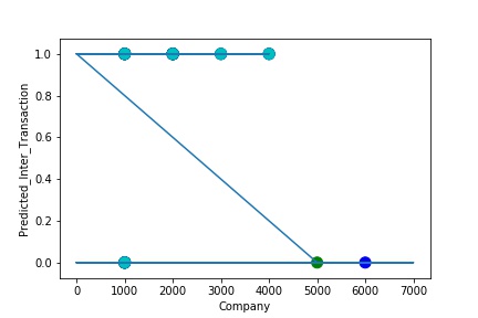
The model is a Regular Fitting Model, when it performs well on training example and also performs well on unseen data. Ideally, the case when the model makes the predictions with 0 error is said to have a best fit on the data. This situation is achievable at a spot between overfitting and under fitting. In order to understand it we will have to look at the performance of our model with the passage of time, while it is learning from training dataset.
A Graph of Company Code vs Predicted Intercompany Transaction (Prediction the Model has made on the Test data)Is Plotted. The Graph shows that our model has learned the underlying pattern in the data quite accurately for which it was trained. The Expected Output Aligns with the Predicted Output. The Model has Achieved Generalization.
A Graph of Company Code vs Predicted Intercompany Transaction (Prediction the Model has made on the Test data) Is again Plotted by Manipulating some of the Pattern in the Data (Ex: Trading Partner in the Below Screenshot). The Model Still is able to Recognize the Right Pattern & Generalize to best fit. (Trading Partner != 0 – IC, Trading Partner = 0 , Non IC)
A GIs again Plotted by Manipulating Pattern in the Data further (Ex: Trading Partner in the Below Screenshot). The Model Still is able to Recognize the Right Pattern & Generalize to best fit. (Trading Partner != 0 – IC, Trading Partner = 0 , Non IC) Graph of Company Code vs Predicted Intercompany Transaction (Prediction the Model has made on the Test data)
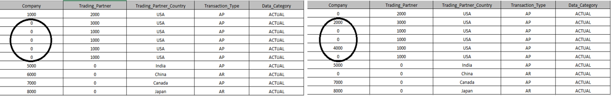
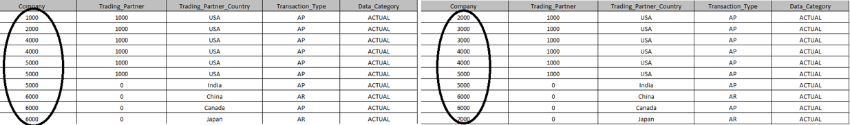
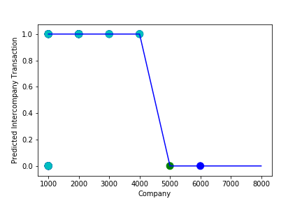
The predictive model is said to be Underfitting, if it performs poorly on training data. Underfitting happens because the model is unable to capture the relationship between the input example and the target variable. It could be because the model is too simple i.e. input features are not expressive enough to describe the target variable well. Underfitting model does not predict the targets in the training data sets very accurately. Underfitting can be avoided by using more data and also reducing the features by feature selection.

A Graph of Company Code vs Predicted Intercompany Transaction (Prediction the Model has made on the Test data) Is Plotted. The Graph shows that our model has not learned the underlying pattern in the data for which it was trained. The Expected Output does not Align with the Predicted Output. The Model has Achieved not achieved Generalization.
A Graph of Company Code vs Predicted Intercompany Transaction (Prediction the Model has made on the Test data) Is again Plotted by Manipulating some of the Pattern in the Data (Ex: Company Code in the Below Screenshot). The Model Still is unable able to recognize the Right Pattern & Generalize to best fit.
A Graph of Company Code vs Predicted Intercompany Transaction (Prediction the Model has made on the Test data) Is again Plotted by Manipulating the Pattern in the Data further. The Model Still is unable able to Recognize the Right Pattern & Generalize to best fit.
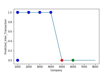
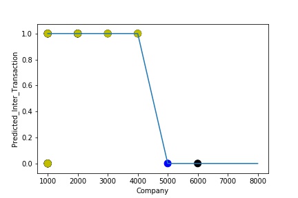
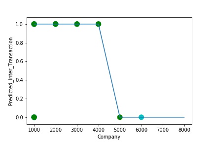
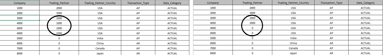
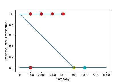
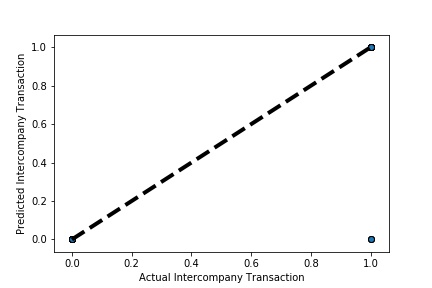
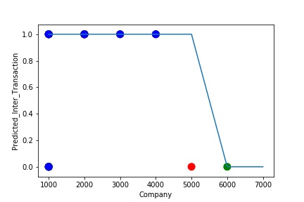
The model is Overfitting, when it performs well on training example but does not perform well on unseen data. It is often a result of an excessively complex model. It happens because the model is memorizing the relationship between the input example (often called X) and target variable (often called y) or, so unable to generalize the data well. Overfitting model predicts the target in the training data set very accurately.

A Graph of Company Code vs Predicted Intercompany Transaction (Prediction the Model has made on the Test data) Is Plotted. The Graph shows that our model has learned the underlying pattern in the data very well for which it was trained. It has learned inaccurate data entries & noise in the data as well. The Expected Output more or less Aligns with the Predicted Output. The Model has Achieved not achieved Generalization.

A Graph of Company Code vs Predicted Intercompany Transaction (Prediction the Model has made on the Test data) Is again Plotted by Manipulating some of the Pattern in the Data (Ex: Company Code in the Below Screenshot). The model has learned the underlying pattern in the data very well again capturing inaccuracy & noise in the data.

A Graph of Company Code vs Predicted Intercompany Transaction (Prediction the Model has made on the Test data) Is again Plotted by Manipulating some of the Pattern in the Data further. The The model has learned the underlying pattern in the data very well again capturing inaccuracy & noise in the data.
Cross-validation is a technique in which we train our model using the subset of the data-set and then evaluate using the complementary subset of the data-set.
A Graph of Actual vs Predicted Intercompany Transaction (Prediction the Model has made on the Test data) Is Plotted. The validation dataset is split into two folds. (EX: 100 Samples into Two folds each folds with 50 Random Samples) The Graph shows that our model has Predicted the Expected Outcome on the Validation data set Accurately. The Expected Output Aligns with the Predicted Output.
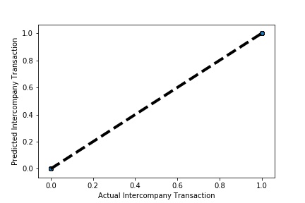
A Graph of Actual vs Predicted Intercompany Transaction (Prediction the Model has made on the Test data) Is Plotted. The validation dataset is split into two folds. (EX: 100 Samples into Two folds each folds with 50 Random Samples) The Graph shows that our model has Predicted the Expected Outcome on the Validation data set Accurately. The Expected Output Aligns with the Predicted Output.
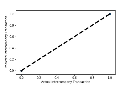
A Graph of Actual vs Predicted Intercompany Transaction (Prediction the Model has made on the Test data) Is Plotted Again by splitting the validation data into 10k folds . (EX: 100 Samples into five folds, each folds with 10 Random Samples) The Graph shows that our model has Predicted the Expected Outcome on the Validation data set Accurately. The Expected Output Aligns with the Predicted Output.
Hyperparameter Optimization or tuning is the problem of choosing a set of optimal hyperparameters for a learning algorithm. The same kind of machine learning model can require different constraints, weights or learning rates to generalize different data patterns. These measures are called hyperparameters, and have to be tuned so that the model can optimally solve the machine learning problem. Hyperparameter optimization finds a tuple of hyperparameters that yields an optimal model which minimizes a predefined loss function on given independent data.

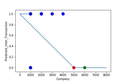
A Graph of Company Code vs Predicted Intercompany Transaction (Prediction the Model has made on the Test data) Is Plotted. In most cases the when the model accuracy is near to 100% it can be improved to 100% by tuning the model parameters. The Below screenshot shoes that the model has 99% accuracy & can be tuned to attain generalization.
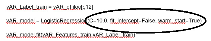
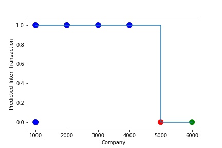
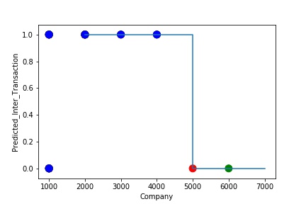
A Graph of Company Code vs Predicted Intercompany Transaction (Prediction the Model has made on the Test data) Is Plotted after tuning some the model Parameter. Ex: regularization parameter C= 1.0 , fit_intercept = False, warm_start= True). The Below screenshot shoes that the model has 100% accuracy & reached generalization.
The model is a Regular Fitting Model, when it performs well on training example & also performs well on unseen data. Ideally, the case when the model makes the predictions with 0 error, is said to have a best fit on the data. This situation is achievable at a spot between overfitting and underfitting. In order to understand it we will have to look at the performance of our model with the passage of time, while it is learning from training dataset.

A Graph of Company Code vs Paired Intercompany Transaction (Prediction the Model has made on the Test data) Is Plotted. The Graph shows that our model has learned the underlying pattern in the data quite accurately for which it was trained. The Expected Output Aligns with the Predicted Output. The Model has Achieved Generalization.

A Graph of Company Code vs Paired Intercompany Transaction (Prediction the Model has made on the Test data) Is again Plotted by Manipulating some of the Pattern in the Data (Ex: Trading Partner). The Model Still is able to Recognize the Right Pattern & Generalize to best fit.

A Graph of Company Code vs Paired Intercompany Transaction (Prediction the Model has made on the Test data) Is again Plotted by Manipulating Pattern in the Data further. The Model Still is able to Recognize the Right Pattern & Generalize to best fit.
The predictive model is said to be Underfitting, if it performs poorly on training data. This happens because the model is unable to capture the relationship between the input example and the target variable. It could be because the model is too simple i.e. input features are not expressive enough to describe the target variable well. Underfitting model does not predict the targets in the training data sets very accurately. Underfitting can be avoided by using more data and also reducing the features by feature selection.
A Graph of Company Code vs Paired Intercompany Transaction (Prediction the Model has made on the Test data) Is Plotted. The Graph shows that our model has not learned the underlying pattern in the data for which it was trained. The Expected Output does not Align with the Predicted Output. The Model has Achieved not achieved Generalization.

A Graph of Company Code vs Predicted Intercompany Transaction (Prediction the Model has made on the Test data) Is again Plotted by Manipulating some of the Pattern in the Data. The Model Still is unable able to recognize the Right Pattern & Generalize to best fit.

A Graph of Company Code vs Paired Intercompany Transaction (Prediction the Model has made on the Test data) Is again Plotted by Manipulating the Pattern in the Data further. The Model Still is unable able to Recognize the Right Pattern & Generalize to best fit.
The model is Overfitting, when it performs well on training example but does not perform well on unseen data. It is often a result of an excessively complex model. It happens because the model is memorizing the relationship between the input example (often called X) and target variable (often called y) or, so unable to generalize the data well. Overfitting model predicts the target in the training data set very accurately.
A Graph of Company Code vs Paired Intercompany Transaction (Prediction the Model has made on the Test data) Is Plotted. The Graph shows that our model has learned the underlying pattern in the data very well for which it was trained. It has learned inaccurate data entries & noise in the data as well. The Expected Output more or less Aligns with the Predicted Output . The Model has Achieved not achieved Generalization.
A Graph of Company Code vs Paired Intercompany Transaction (Prediction the Model has made on the Test data) Is again Plotted by Manipulating some of the Pattern in the Data. The model has learned the underlying pattern in the data very well again capturing inaccuracy & noise in the data.
A Graph of Company Code vs Predicted Intercompany Transaction (Prediction the Model has made on the Test data) Is again Plotted by Manipulating some of the Pattern in the Data further. The model has learned the underlying pattern in the data very well again capturing inaccuracy & noise in the data.
Cross-validation is a technique in which we train our model using the subset of the data-set and then evaluate using the complementary subset of the dataset.

A Graph of Actual vs Paired Intercompany Transaction (Prediction the Model has made on the Test data) Is Plotted. The validation dataset is split into two folds. (EX: 100 Samples into Two folds each folds with 50 Random Samples) The Graph shows that our model has Predicted the Expected Outcome on the Validation data set Accurately. The Expected Output Aligns with the Predicted Output.

A Graph of Actual vs Predicted Intercompany Transaction (Prediction the Model has made on the Test data) Is Plotted Again by splitting the validation data into 5k folds . (EX: 100 Samples into five folds, each folds with 20 Random Samples) The Graph shows that our model has Predicted the Expected Outcome on the Validation data set Accurately. The Expected Output Aligns with the Predicted Output.

A Graph of Actual vs Predicted Intercompany Transaction (Prediction the Model has made on the Test data) Is Plotted Again by splitting the validation data into 10k folds . (EX: 100 Samples into five folds, each folds with 10 Random Samples) The Graph shows that our model has Predicted the Expected Outcome on the Validation data set Accurately. The Expected Output Aligns with the Predicted Output.
Hyperparameter Optimization or tuning is the problem of choosing a set of optimal hyperparameters for a learning algorithm. The same kind of machine learning model can require different constraints, weights or learning rates to generalize different data patterns. These measures are called hyperparameters and must be tuned so that the model can optimally solve the machine learning problem. Hyperparameter optimization finds a tuple of hyperparameters that yields an optimal model which minimizes a predefined loss function on given independent data.

A Graph of Company Code vs Paired Intercompany Transaction (Prediction the Model has made on the Test data) Is Plotted. In most cases the when the model accuracy is near to 100% it can be improved to 100% by tuning the model parameters. The Below screenshot shoes that the model has 99% accuracy & can be tuned to attain generalization.

A Graph of Company Code vs Paired Intercompany Transaction (Prediction the Model has made on the Test data) Is Plotted after tuning some the model Parameter. Ex: regularization parameter C= 1.0 , fit_intercept = False, warm_start= True). The Below screenshot shoes that the model has 100% accuracy & reached generalization.
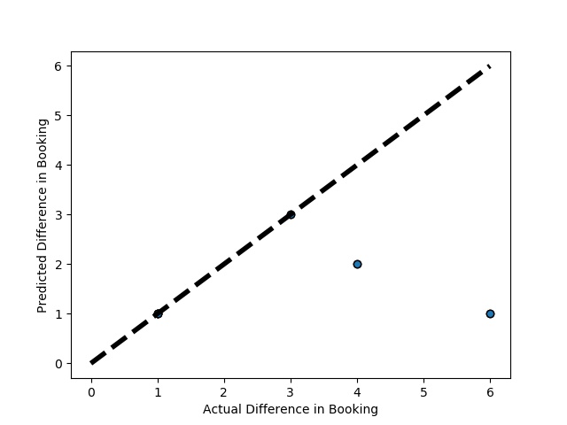
The model is a Regular Fitting Model, when it performs well on training example & also performs well on unseen data. Ideally, the case when the model makes the predictions with 0 error, is said to have a best fit on the data. This situation is achievable at a spot between overfitting and underfitting. In order to understand it we will have to look at the performance of our model with the passage of time, while it is learning from training dataset.
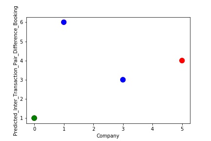
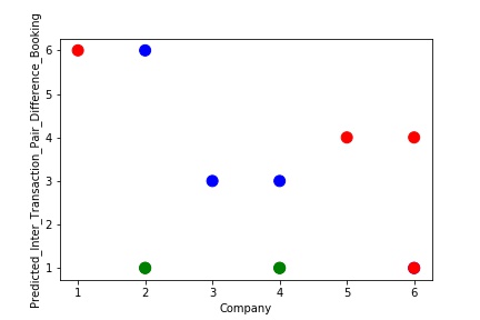
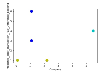
A Graph of Company Code vs Paired Intercompany Transaction for Diff in Booking (Prediction the Model has made on the Test data) Is Plotted. The Graph shows that our model has learned the underlying pattern in the data quite accurately for which it was trained. The Expected Output Aligns with the Predicted Output. The Model has Achieved Generalization.
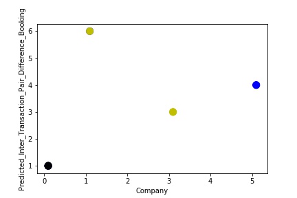
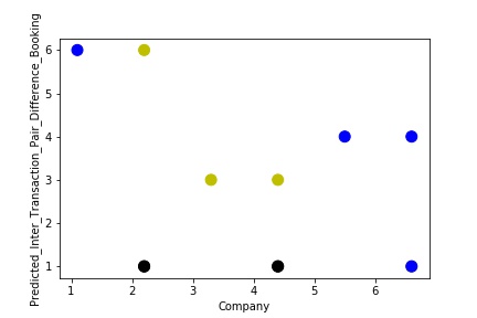
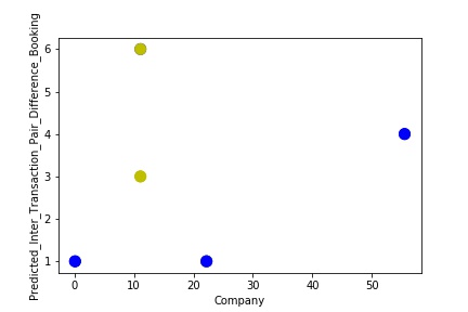
A Graph of Company Code vs Paired Intercompany Transaction for Diff in Booking (Prediction the Model has made on the Test data) Is again Plotted by Manipulating some of the Pattern in the Data (Ex: Trading Partner). The Model Still is able to Recognize the Right Pattern & Generalize to best fit.
A Graph of Company Code vs Paired Intercompany Transaction for Diff in Booking (Prediction the Model has made on the Test data) Is again Plotted by Manipulating Pattern in the Data further. The Model Still is able to Recognize the Right Pattern & Generalize to best fit.
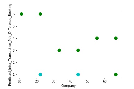
The predictive model is said to be Underfitting, if it performs poorly on training data. This happens because the model is unable to capture the relationship between the input example and the target variable. It could be because the model is too simple i.e. input features are not expressive enough to describe the target variable well. Underfitting model does not predict the targets in the training data sets very accurately. Underfitting can be avoided by using more data and also reducing the features by feature selection.
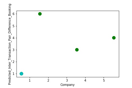
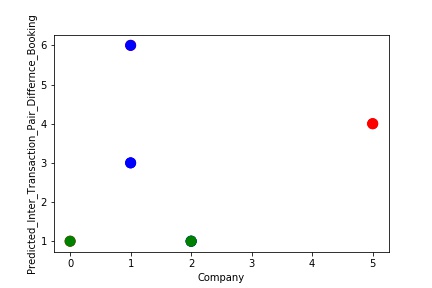
A Graph of Company Code vs Paired Intercompany Transaction for diff in booking (Prediction the Model has made on the Test data) Is Plotted. The Graph shows that our model has not learned the underlying pattern in the data for which it was trained. The Expected Output does not Align with the Predicted Output. The Model has Achieved not achieved Generalization.
A Graph of Company Code vs Predicted Intercompany Transaction for diff in booking (Prediction the Model has made on the Test data) Is again Plotted by Manipulating some of the Pattern in the Data. The Model Still is unable able to recognize the Right Pattern & Generalize to best fit.
A Graph of Company Code vs Paired Intercompany Transaction for diff in booking (Prediction the Model has made on the Test data) Is again Plotted by Manipulating the Pattern in the Data further. The Model Still is unable able to Recognize the Right Pattern & Generalize to best fit.
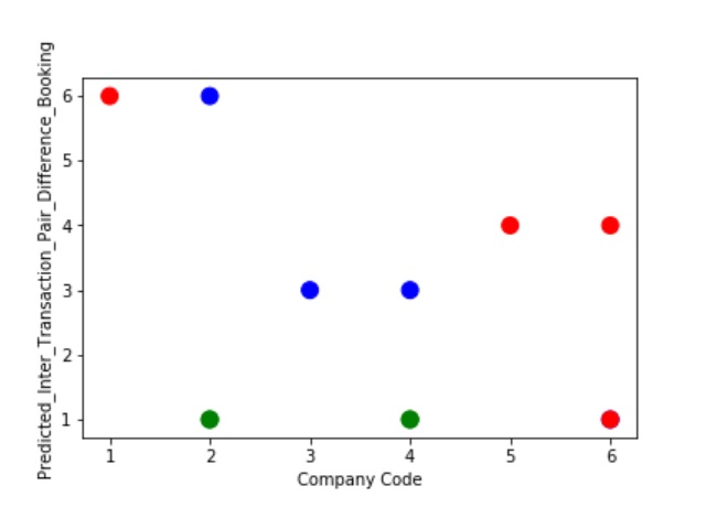
The model is Overfitting, when it performs well on training example but does not perform well on unseen data. It is often a result of an excessively complex model. It happens because the model is memorizing the relationship between the input example (often called X) and target variable (often called y) or, so unable to generalize the data well. Overfitting model predicts the target in the training data set very accurately.
A Graph of Company Code vs Paired Intercompany Transaction for diff in booking (Prediction the Model has made on the Test data) Is Plotted. The Graph shows that our model has learned the underlying pattern in the data very well for which it was trained. It has learned inaccurate data entries & noise in the data as well. The Expected Output more or less Aligns with the Predicted Output . The Model has Achieved not achieved Generalization.
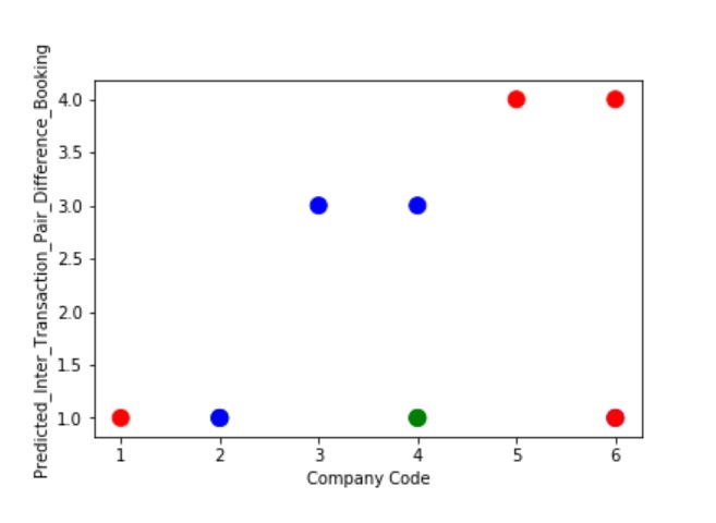
A Graph of Company Code vs Paired Intercompany Transaction for diff in booking (Prediction the Model has made on the Test data) Is again Plotted by Manipulating some of the Pattern in the Data. The model has learned the underlying pattern in the data very well again capturing inaccuracy & noise in the data.
A Graph of Company Code vs Predicted Intercompany Transaction for diff in booking (Prediction the Model has made on the Test data) Is again Plotted by Manipulating some of the Pattern in the Data further. The model has learned the underlying pattern in the data very well again capturing inaccuracy & noise in the data.
Cross-validation is a technique in which we train our model using the subset of the data-set and then evaluate using the complementary subset of the data-set.
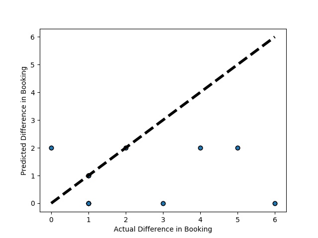
A Graph of Actual vs Paired Intercompany Transaction for diff in booking (Prediction the Model has made on the Test data) Is Plotted. The validation dataset is split into two folds. (EX: 100 Samples into Two folds each folds with 50 Random Samples) The Graph shows that our model has Predicted the Expected Outcome on the Validation data set Accurately. The Expected Output Aligns with the Predicted Output.
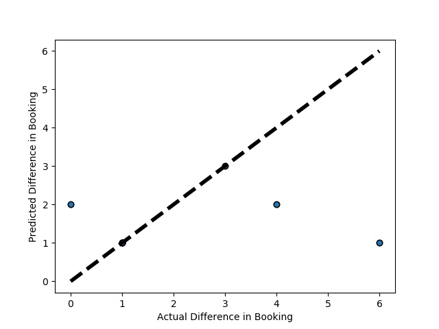
A Graph of Actual vs Predicted Intercompany Transaction for diff in booking (Prediction the Model has made on the Test data) Is Plotted Again by splitting the validation data into 5k folds . (EX: 100 Samples into five folds, each folds with 20 Random Samples) The Graph shows that our model has Predicted the Expected Outcome on the Validation data set Accurately. The Expected Output Aligns with the Predicted Output.
A Graph of Actual vs Predicted Intercompany Transaction for diff in booking (Prediction the Model has made on the Test data) Is Plotted Again by splitting the validation data into 10k folds . (EX: 100 Samples into five folds, each folds with 10 Random Samples) The Graph shows that our model has Predicted the Expected Outcome on the Validation data set Accurately. The Expected Output Aligns with the Predicted Output.
Hyperparameter Optimization or tuning is the problem of choosing a set of optimal hyperparameters for a learning algorithm. The same kind of machine learning model can require different constraints, weights or learning rates to generalize different data patterns. These measures are called hyperparameters, and have to be tuned so that the model can optimally solve the machine learning problem. Hyperparameter optimization finds a tuple of hyperparameters that yields an optimal model which minimizes a predefined loss function on given independent data.
A Graph of Company Code vs Paired Intercompany Transaction for diff in booking (Prediction the Model has made on the Test data) Is Plotted. In most cases the when the model accuracy is near to 100% it can be improved to 100% by tuning the model parameters. The Below screenshot shoes that the model has 99% accuracy & can be tuned to attain generalization.
A Graph of Company Code vs Paired Intercompany Transaction for diff in booking (Prediction the Model has made on the Test data) Is Plotted after tuning some the model Parameter. Ex: regularization parameter C= 1.0 , fit_intercept = False, warm_start= True). The Below screenshot shoes that the model has 100% accuracy & reached generalization.
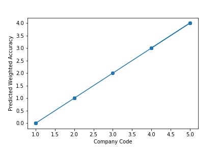
The model is a Regular Fitting Model, when it performs well on training example & also performs well on unseen data. Ideally, the case when the model makes the predictions with 0 error, is said to have a best fit on the data. This situation is achievable at a spot between overfitting and underfitting. In order to understand it we will have to look at the performance of our model with the passage of time, while it is learning from training dataset.

A Graph of Company Code vs Predicted Weighted Accuracy of Intercompany Transaction (Prediction the Model has made on the Test data) is Plotted. The Graph shows that our model has learned the underlying pattern in the data quite accurately for which it was trained. The Expected Output Aligns with the Predicted Output. The Model has Achieved Generalization.
A Graph of Company Code Predicted Weighted Accuracy of Intercompany Transaction (Prediction the Model has made on the Test data) Is again Plotted by Manipulating some of the Pattern in the Data (Ex: Trading Partner). The Model Still is able to Recognize the Right Pattern & Generalize to best fit.

A Graph of Company Code vs Predicted Weighted Accuracy of Intercompany Transaction (Prediction the Model has made on the Test data) Is again Plotted by Manipulating Pattern in the Data further. The Model Still is able to Recognize the Right Pattern & Generalize to best fit.
The predictive model is said to be Underfitting, if it performs poorly on training data. This happens because the model is unable to capture the relationship between the input example and the target variable. It could be because the model is too simple i.e. input features are not expressive enough to describe the target variable well. Underfitting model does not predict the targets in the training data sets very accurately. Underfitting can be avoided by using more data and also reducing the features by feature selection.

A Graph of Company Code vs Predicted Weighted Accuracy of Intercompany Transaction (Prediction the Model has made on the Test data) is Plotted. The Graph shows that our model has not learned the underlying pattern in the data for which it was trained. The Expected Output does not Align with the Predicted Output. The Model has Achieved not achieved Generalization.

A Graph of Company Code vs Predicted Weighted Accuracy of Intercompany Transaction (Prediction the Model has made on the Test data) Is again Plotted by Manipulating some of the Pattern in the Data. The Model Still is unable able to recognize the Right Pattern & Generalize to best fit.
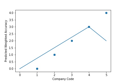
A Graph of Company Code vs Predicted Weighted Accuracy of Intercompany Transaction (Prediction the Model has made on the Test data) Is again Plotted by Manipulating the Pattern in the Data further. The Model Still is unable able to Recognize the Right Pattern & Generalize to best fit.
The model is Overfitting, when it performs well on training example but does not perform well on unseen data. It is often a result of an excessively complex model. It happens because the model is memorizing the relationship between the input example (often called X) and target variable (often called y) or, so unable to generalize the data well. Overfitting model predicts the target in the training data set very accurately.
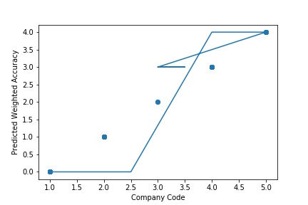
A Graph of Company Code vs Predicted Weighted Accuracy of Intercompany Transaction (Prediction the Model has made on the Test data) is Plotted. The Graph shows that our model has learned the underlying pattern in the data very well for which it was trained. It has learned inaccurate data entries & noise in the data as well. The Expected Output more or less Aligns with the Predicted Output. The Model has Achieved not achieved Generalization.
A Graph of Company Code vs Predicted Weighted Accuracy of Intercompany Transaction (Prediction the Model has made on the Test data) Is again Plotted by Manipulating some of the Pattern in the Data. The model has learned the underlying pattern in the data very well again capturing inaccuracy & noise in the data.
A Graph of Company Code vs Predicted Weighted Accuracy of Intercompany Transaction (Prediction the Model has made on the Test data) Is again Plotted by Manipulating some of the Pattern in the Data further. The model has learned the underlying pattern in the data very well again capturing inaccuracy & noise in the data.
Cross-validation is a technique in which we train our model using the subset of the data-set and then evaluate using the complementary subset of the data-set.
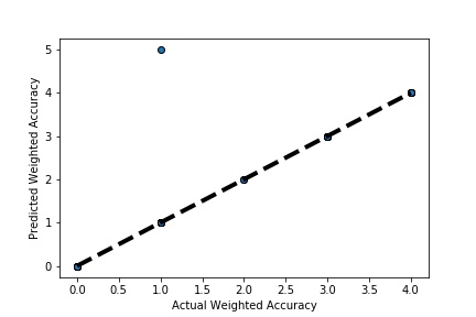
A Graph of Actual vs Predicted Weighted Accuracy of Intercompany Transaction (Prediction the Model has made on the Test data) Is Plotted. The validation dataset is split into two folds. (EX: 100 Samples into Two folds each folds with 50 Random Samples) The Graph shows that our model has Predicted the Expected Outcome on the Validation data set Accurately. The Expected Output Aligns with the Predicted Output.
A Graph of Actual vs Predicted Weighted Accuracy of Intercompany Transaction (Prediction the Model has made on the Test data) Is Plotted Again by splitting the validation data into 5k folds. (EX: 100 Samples into five folds, each folds with 20 Random Samples) The Graph shows that our model has Predicted the Expected Outcome on the Validation data set Accurately. The Expected Output Aligns with the Predicted Output.
A Graph of Actual vs Predicted Weighted Accuracy of Intercompany Transaction (Prediction the Model has made on the Test data) Is Plotted Again by splitting the validation data into 10k folds. (EX: 100 Samples into five folds, each folds with 10 Random Samples) The Graph shows that our model has Predicted the Expected Outcome on the Validation data set Accurately. The Expected Output Aligns with the Predicted Output.
Hyperparameter Optimization or tuning is the problem of choosing a set of optimal hyperparameters for a learning algorithm. The same kind of machine learning model can require different constraints, weights or learning rates to generalize different data patterns. These measures are called hyperparameters, and have to be tuned so that the model can optimally solve the machine learning problem. Hyperparameter optimization finds a tuple of hyperparameters that yields an optimal model which minimizes a predefined loss function on given independent data.

A Graph of Company Code vs Predicted Weighted Accuracy of Intercompany Transaction (Prediction the Model has made on the Test data) Is Plotted. In most cases the when the model accuracy is near to 100% it can be improved to 100% by tuning the model parameters. The Below screenshot shoes that the model has 99% accuracy & can be tuned to attain generalization.
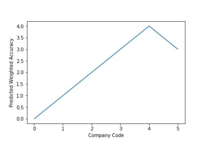
A Graph of Company Code vs Predicted Weighted Accuracy of Intercompany Transaction (Prediction the Model has made on the Test data) Is Plotted after tuning some the model Parameter. Ex: regularization parameter C= 1.0 , fit_intercept = False, warm_start= True). The Below screenshot shoes that the model has 100% accuracy & reached generalization.
All software and hardware used or referenced in this white paper belong to their respective vendor. We have developed this functional and technical artifacts based on our development infrastructure and these artifacts may or may not work on others systems and technical infrastructure. We are not liable for any direct or indirect problems caused to the users using this guide.

Requestor with a valid email and phone will get a copy of this white paper.